Red Bull Air Race is an international series of air races in which competitors have to navigate a challenging obstacle course in the fastest time possible. Pilots fly individually against the clock and have to complete tight turns through a slalom course consisting of pylons, known as “Air Gates”, achieving speeds of up to 420 km/h and sustained accelerations of more than 10 G.
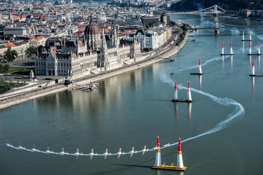
Figure 1 - Red Bull Air Race 2016 in Budapest
Participant teams usually spend a significant amount of time trying to predict optimal aircraft trajectories to follow for each track, in an effort to achieve the fastest possible lap times.
In early 2018 I started working in a personal project to develop an analysis tool which enabled a temporal-space study of optimal trajectories for different race tracks.
The problem is not trivial. Let’s start from the beginning.
Table of Contents
- What is the objective?
- A simplistic approach
- More complex approaches
- Aerodynamic model
- Aircraft Kinematics
- The tool
- Source Code
- References
What is the objective?
Races usually have two types of obstacles: Airgates of single or double pylons. Pilots are required to fly near the single pylons and between the double pylons, following a predetermined route as fast as possible.
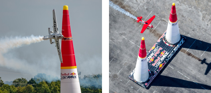
Figure 2 - Single pylon (left) and double pylons or gates (right)
There exist several restrictions to take into consideration, including the following:
- Pilots must fly through the double pylon air gates in level flight. This is, the aircraft has to be flying straight when passing through these airgates.
- Pilots must fly through the airgates while inside the altitude range indicated by the red bands in the pylons.
- Aircraft must never cross any safety line, which delimit the compulsory safety flight area.
- Aircraft must not surpass the acceleration limit of 10 G.
- Aircraft must not start the race with a velocity higher than 200 knots.
How could we approach this problem?
A simplistic approach
This is an optimization problem with several types of constraints. We need to find a way to simplify the problem in order to reduce complexity.
Let’s try a simple approach by making some hypotheses:
- Aircraft trajectories are smooth because the aircraft movement is always restricted by inertia. This means these trajectories can be approximated by some type of mathematical curve.
- This kind of air races usually take place in 2D planes, since aircraft fly most of the time at the same altitude. Let’s forget about the third degree of freedom for now.
- Aircraft longitudinal acceleration when flying straight is mostly dictated by the engine thrust and its aerodynamic resistance.
- Aerodynamic resistance grows exponentially with aircraft lift.
- When an aircraft is performing a turn, lift needs to be increased in order to maintain altitude. Turning angle (roll) is dictated by the curvature of the aircraft trajectory.
Given this statements, a direct relation can be extrapolated between the trajectory local curvature and the aircraft longitudinal acceleration at that location.
But what type of mathematical curve may an aircraft trajectory look like? One option is a cubic spline.
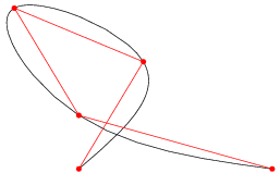
Figure 3 - Cubic spline
A cubic spline is a spline constructed of piecewise third-order polynomials which pass through a set of $m$ control points. The second derivative of each polynomial is commonly set to zero at the endpoints, since this provides a boundary condition that completes the system of $m-2$ equations. This produces a so-called “natural” cubic spline and leads to a simple tridiagonal system which can be solved easily to give the coefficients of the polynomials [1].
The trajectories can be approximated by bidimensional splines parametrized in two degrees of freedom $x$ and $y$. This is, there’s a third degree polynomial defining $x{\left (t \right)}$, and a third degree polynomial defining $y{\left (t \right)}$. These curves provide a good approximation of the real trajectories. Curves of higher order could approach the trajectories more precisely, but they unnecessarily increase the complexity of the optimization problem and increase the probability of convergence to a local minimum instead of a global minimum. Order 3 polynomials provide a good balance between complexity and precision.
Now, let’s analyse the effect of turning angle (roll) in an aircraft lift while flying at the same altitude.
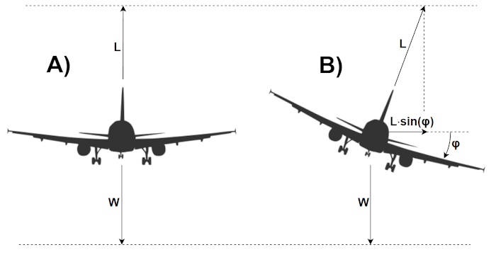
Figure 4 - Effect of roll on lift during level flight
When an aircraft is flying straight (4A), it’s weight, $W$, needs to be compensated by the generated lift, $L$. However, when an aircraft is turning (4B), lift needs to be increased in order to be able to compensate the weight. The lift component in the vertical axis compensates the aircraft weight. This component is $ L{\cdot}\cos \left (\varphi \right) $. An additional component is generated in the horizontal axis, $ L{\cdot}\sin \left (\varphi \right) $. This component represents a centripetal force which causes the aircraft trajectory azimuth to change, achieving the turn.
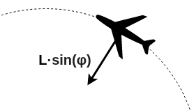
Figure 5 - Centripetal force during a turn
The radius of curvature is dictated by current velocity and the aircraft weight. The centripetal force in a moving body can be defined by
Where $R$ is the local radius of curvature. The lift component in the vertical axis needs to compensate the aircraft weight in order to maintain altitude.
These two equations can be combined to form
Given that
and that local curvature in a curve is defined as the inverse of the local radius
then
This equation will be useful when we derive another set of equations, corresponding to the longitudinal degree of freedom.
Local curvature of a bidimensional spline, which is parametrized in two degrees of freedom $x{\left (t \right)}$ and $y{\left (t \right)}$, can be calculated using the following formula.
Piecewise splines parametrized with third order polynomials are only continuous up until the first derivative. This means that there are discontinuities in the spline curvature at the control points joining each section of the spline. However this is not a problem for aerobatic planes, since their high manoeuvrability enables them to adapt closely to these trajectories even in the control point sections.
Up until this point, the only mathematical concepts used where geometric and trigonometric relations, as well as the concept of force equilibrium and the definitions of centripetal force and curvature of a parametrized curve.
Now we need to take into account the aerodynamic forces. We will model lift, $L$, and drag, $D$, forces using the following equations [2].
Where $q$ is the dynamic pressure, defined as $\frac{1}{2}{\cdot}\rho{\cdot}V^2$, being $\rho$ the air density and $V$ the total velocity of the aircraft. Variable $S$ corresponds to the wing reference surface. Variables $C_L$ and $C_D$ correspond to the lift coefficient and drag coefficient respectively. We will define those as
Where $\alpha$ refers to the aircraft angle of attack, $C_{L_0}$ and ${C_{D_0}}$ refer to the lift and drag coefficients at zero angle of attack, and $C_{L_{\alpha}}$ and ${K}$ are aerodynamic parameters dependant on the specific aircraft.
Aircraft acceleration, $a$, can be modelled using Newton’s first law of motion, having into account the vehicle mass, $m$.
We can discretize the trajectory of the aircraft along the spline in small sectors. Considering $V_i$ the velocity at the start of a sector, $V_{med}$ the velocity at the middle point of the sector, and $l$ the length of the sector, combining equations (6-9) we can approximate the acceleration at each sector by:
Where
The solution of system of equations (11) and (12) for variable $V_{med}$ in order to find the medium velocity at each timestep reduces to a quartic equation, which can be solved using Ferrari’s formula.
Where coefficients $a$, $b$, $c$, $d$ and $e$ result in
Ferrari’s formula uses the following relations which provide the analytic solution of the quartic equation [3].
We are interested in the biggest real solution to the polynomic equation.
Equation 19 defines the medium velocity at each small section of the spline as a function of the initial velocity at that section, the arclength of the section, aircraft thrust, local curvature of the spline, aerodynamic parameters such as $C_{D_0}$, $S$ or $K$ and physical properties of the system such as air density, acceleration due to gravity and the mass of the aircraft. Therefore, an iterative process can be made in order to calculate the velocity along an entire bidimensional spline. This process is similar to an integration of this variable along the spline, and if the section arclength is set to be sufficiently small then the associated errors of the numerical iterative process would become negligible.
Using this pipeline one could perform an optimization process in which bidimensional splines are generated to pass through $m$ control points (race pylons) and a total time is calculated and associated to each of those splines, optimising the spline parameters in order to minimize the total trajectory associated time. The optimization should find a global minimum, not local. The complexity of the problem may originate many local minimums which could be a problem if using a local optimizer and the initial conditions are not close enough to the global minimum.
The global optimizer I chose to solve this problem is a Genetic Algorithm. A genetic algorithm (GA) is a method for solving both constrained and unconstrained optimization problems based on a natural selection process that mimics biological evolution. The algorithm repeatedly modifies a population of individual solutions. At each step, the genetic algorithm randomly selects individuals from the current population and uses them as parents to produce the children for the next generation. Over successive generations, the population “evolves” toward an optimal solution. You can apply the genetic algorithm to solve problems that are not well suited for standard optimization algorithms, including problems in which the objective function is discontinuous, nondifferentiable, stochastic, or highly nonlinear [4]. Using this solver, it is easier to converge to the global minimum instead of getting stuck in a not globally optimal local minimum.
I implemented this pipeline in the numerical computing environment MATLAB®. A link to the actual code is available in Source Code section. I tested the tool with a simple air race track example, which can be observed in the figure below.
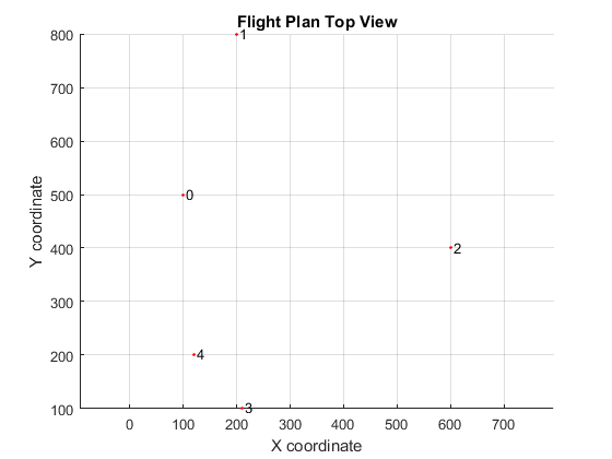
Figure 6 - Track waypoints
The track includes five control waypoints. In order to solve the problem it is necessary to impose a trajectory heading at each waypoint, where we can define the heading as $\arctan{\left(y’/x’ \right)}$. This way, the order complexity of the problem reduces to the number of waypoints, $m$. The global minimum total time trajectory calculated by the tool can be observed in the following figures.
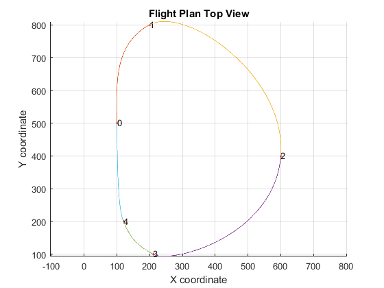
Figure 7 - Trajectory solution
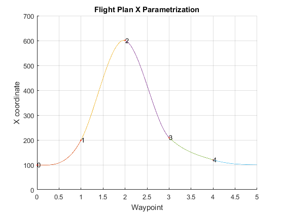
Figure 8 - Solution X parametrization
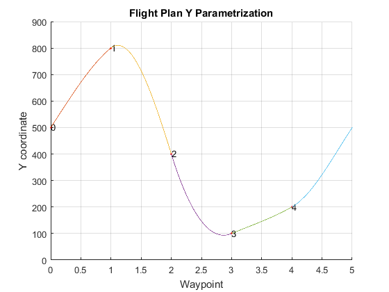
Figure 9 - Solution Y parametrization
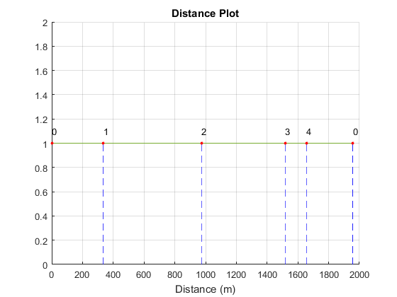
Figure 10 - Flight distance along trajectory
This approach can be used to provide first approximations of track time, but is not precise enough to be practical in real races. More elements need to be added in order to improve the pipeline, such as adding the third degree of freedom (altitude), taking into account more aerodynamic coefficients like the lift coefficient due to angle of attack, $C_{L_\alpha}$, or modelling these coefficients as a function of velocity using look-up tables.
More complex approaches
The solution to this problem needs to take into account many elements. First of all the dynamics associated with a moving vehicle on Earth. In other hand the own vehicle aerodynamics and thrust dynamics, and their relations with the vehicle control surfaces. Also, the point constraints associated with the control points (roll limits, velocity limits…), as well as the path constraints requirements along the entire trajectory (max G-force limits, position constraints inside the safety flight zone…).
One could try to apply a deep reinforcement learning method, like Deep Q-Learning. The goal of Q-learning is to learn a policy, which tells an agent what action to take under what circumstances. It does not require a model of the environment, and it can handle problems with stochastic transitions and rewards, without requiring adaptations [5]. However, the degree of complexity of the problem in hand is excessively high for this method. The space of possible states and actions is huge, making it impractical to apply this technique to optimize the entire trajectory.
Another approach to this optimal control problem is based on a technique called direct collocation. Direct collocation methods work by approximating the state and control trajectories using polynomial splines [6]. These methods are sometimes referred to as direct transcription. This technique can be used to transcribe the aicraft dynamics and all constraints into a problem which can be solved using nonlinear programming. In mathematics, nonlinear programming (NLP) is the process of solving an optimization problem where some of the constraints or the objective function are nonlinear.
In order to implement this technique, I used the library falcon.m [7]. This library is a free optimal control tool developed at the Institute of Flight System Dynamics of the Technical University of Munich (TUM). It provides a MATLAB® class library which allows to set-up, solve and analyze optimal control problems using numerical optimization methods. The code is optimized for usability and performance and enables the solution of high fidelity real-life optimal control problems with ease.
Aerodynamic model
A precise dynamic model is essential for this project. This section presents a complete aerodynamic model which can be used to model the aircraft.
Vehicle aerodynamics are modelled by taking into account forces and moments. On textbooks on aerodynamics [8] it is shown that, for a body of given shape with a given orientation to the freestream flow, the forces and moments are proportional to the product of freestream mass density, $\rho$, the square of the freestream airspeed, $V$, and a characteristic area of the body. When modelling aircraft aerodynamics, the characteristic area of the body is typically selected as the wing reference surface, $S$. The product of the first two quantities has the dimensions of pressure and it is convenient to define the dynamic pressure, $q$, by
We are now in a position to write down the mathematical models for the magnitudes of the forces and moments. The forces and moments acting on the complete aircraft are defined in terms of dimensionless aerodynamic coefficients in equations 22 and 23 respectively. Moment nondimensionalization is usually performed with additional parameters like wingspan, $b$, or wing mean chord, $c$.
Aerodynamic forces
Aerodynamic moments
The aircraft aerodynamic coefficients are, in practice, specified as functions of the aerodynamic angles, velocity, and altitude. In addition, control surface deflections and propulsion system effects cause changes in the coefficients. A control surface deflection, $\delta_s$, effectively changes the camber of a wing, which changes the lift, drag, and moment.
Aerodynamic angles is the name given to two different angles:
The angle of attack, $\alpha$, specifies the angle between the chord line of the wing of a fixed-wing aircraft and the freestream velocity vector. It is the primary parameter in longitudinal stability considerations.
The sideslip angle, $\beta$, specifies the angle between the freestream velocity vector to the longitudinal axis of the vehicle when projected in the horizontal plane. The sideslip angle is essentially the directional angle of attack of the airplane. It is the primary parameter in directional stability considerations.
Angle of attack and sideslip angle definitions are schematized in figures 11 and 12.
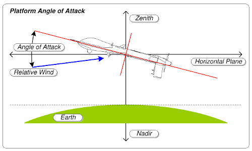
Figure 11 - Angle of attack
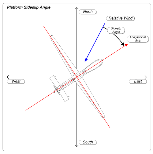
Figure 12 - Sideslip angle
Aerodynamic angles can be defined as a function of the velocity components in body-axes coordinate system
Consequently, force and moment coefficients can be approximated by equations 25 and 26 respectively, which are defined below.
Aerodynamic forces coefficients
Aerodynamic moments coefficients
Aerodynamic derivative $C_{x_y}$ provides information about the effect on the variable $x$ caused by a unitary increment in the variable $y$. Aerodynamic derivatives $C_{L_0}$ and $C_{D_0}$ are called zero angle of attack lift and parasite drag respectively, and they represent the lift and drag contribution which is not due to any other variable and is present even at zero angle of attack.
The coefficients shown in equations 25 and 26 are usually named aerodynamic coefficients or aerodynamic derivatives, and they can be classified into three different groups:
Stability derivatives
Control derivatives
Damping derivatives
Note that terms concerning damping derivatives are always nondimensionalized in the moment coefficients equations. The nondimensionalization factor is dependant on the reference axis.
Aircraft Kinematics
This section includes the aircraft kinematic equations which model the derivatives of the aircraft states in terms of the resulting forces and moments of the aerodynamic model, and of the states themselves [2].
Force equations
Kinematic equations
Moment equations
Navigation equations
These equations, in combination with the aerodynamics equations, model the complete aircraft dynamics (dynamic states) as a state of the control surfaces and the dynamic states themselves.
Simplified model
Library falcon.m uses the software package Ipopt for large-scale nonlinear optimization [9]. This software is designed to find local solutions of mathematical optimization problems for minimization of an objective function subject to constraints. It is written in C++ for efficiency. The dynamic model described in the previous sections is complex, so the solution space tends to have numerous local solutions. This is a problem because Ipopt is a tool for local optimization, not global. In order to smooth the solution space and eliminate numerous local solutions, a simpler approximation is proposed. The motion of the center of mass of an aircraft can be alternatively described [10][11] by the following equations.
The quaternions must satisfy the constraint
This equations of motion are valid for flat, nonrotating earth and for flight without sideforces and with constant mass. The assumption is made that the flight path angles (azimuth, $\chi$, and flight path angle with respect to the horizontal plane, $\gamma$) are approximately equal to the euler angles components yaw, $\psi$, and pitch, $\theta$. We can approximate lift and drag by
The quaternions are related to the euler angles [12] by
or
This equations of motion result to be much simpler than the complete aerodynamics and kinematics systems described in previous sections. This sacrifices model accuracy in turn for a smoother solution space which increases the probability of finding a global minimum if the initial conditions are set to be close enough, given that this solution space has less local minimums where the solver can converge.
The tool
The quaternion-based model can be implemented as an objective function in falcon.m.
function [states_dot] = dyn_complete(states, controls)
% model interface created by falcon.m

% Extract states
V = states(1);
q0 = states(2);
q1 = states(3);
q2 = states(4);
q3 = states(5);

% Extract controls
alpha = controls(1);
T = controls(2);
p = controls(3);

% Constants
m = 750;
g = 9.8056;
rho = 1.225;
S = 9.84;
Clalpha = 5.7;
K = 0.18;
Cd0 = 0.0054;
Cl0 = 0.1205;
Cdp = 0.05;

% Dynamic model
Cl = Clalpha.*alpha + Cl0;
L = 0.5.*rho.*V.^2.*S.*Cl;
D = 0.5.*rho.*V.^2.*S.*(Cd0+K.*Cl.^2+Cdp*abs(p));
q = (T.*sin(alpha)+L-m.*g.*(q0.^2-q1.^2-q2.^2+q3.^2))./(m.*V);
r = (2.*m.*g.*(q0.*q1+q2.*q3))./(m.*V);
V_dot = (T.*cos(alpha)-D+2.*m.*g.*(q1.*q3-q0.*q2))./m;
q0_dot = -0.5.*(q1.*p+q2.*q+q3.*r);
q1_dot =  0.5.*(q0.*p+q2.*r-q3.*q);
q2_dot =  0.5.*(q0.*q+q3.*p-q1.*r);
q3_dot =  0.5.*(q0.*r+q1.*q-q2.*p);
x_dot = V.*(q0.^2+q1.^2-q2.^2-q3.^2);
y_dot = 2.*V.*(q0.*q3+q1.*q2);
h_dot = 2.*V.*(q0.*q2-q1.*q3);
states_dot = [T_dot; V_dot; alpha_dot; q0_dot; q1_dot; q2_dot; q3_dot; x_dot; y_dot; h_dot];

end
The tool falcon.m uses Matlab Symbolic Toolbox to find the analytic gradients of the objective function. This task can become complex if the entire dynamic model is considered. In order to facilitate the gradient calculation, the quaternion-based model can be divided into small sections, each of which has an easier gradient calculation and can be all concatenated when finished. This divide and conquer strategy speeds up execution time and decreases the probability of not finding a solution.
Next, the constraints should be implemented into the tool. Constraints are classified in two types:
Point boundaries: These are only applied in the initial and final points of the segments (control waypoints). Here we can include the position constraints to pass through/near the pylons and the attitude constraints to pass through the double pylons at level flight.
Path constraints: These are applied along the entire segments. Here we can include the acceleration limits, the position limits to fly inside the safety area, and the requirement that the norm of the quaternion components is always 1. This last constraint helps to correct the possible numerical errors accumulated during the propagation.
The complete optimal control problem is implemented in two separate routines:
Segment optimization: Optimization for a single trajectory segment joining a control waypoint with the next one.
Trajectory optimization: Trajectory segments are optimized sequentially in order to obtain an optimal control strategy for the entire trajectory. Each new segment has the initial conditions resulting from the final conditions of the previous segment. This logic is not optimal, since the solver is optimizing each segment independently of the future segments. Nevertheless, the results are almost optimal given that the segments are significantly big. A future tool improvement could be to connect each segment optimization pipeline in order to have into account the $N$ following segments. falcon.m already implements this functionality to connect individual optimization problems.
FlightGear graphical visualization
In order to provide graphical visualization of the resulting trajectories, compatibility with FlightGear open source flight simulator has been implemented in the tool. This also allows to manually test the dynamic model using a Joystick. The graphical visualization engine receives the aircraft’s position and attitude from the MATLAB® tool via a UDP socket at 60 Hz.

Figure 13 - FlighGear graphical visualization (view from vertical stabilizer)
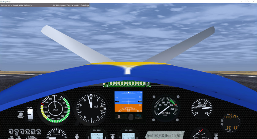
Figure 14 - FlighGear graphical visualization (cockpit view)
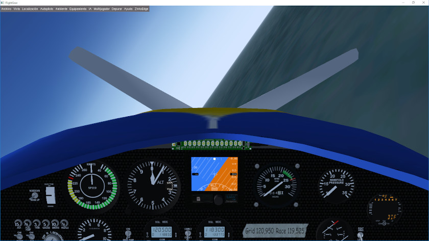
Figure 15 - FlighGear graphical visualization (cockpit view)
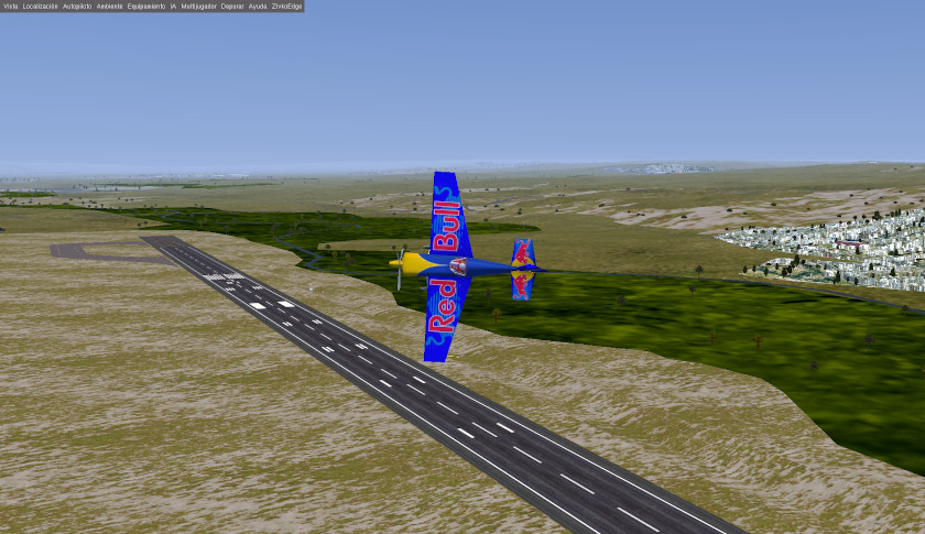
Figure 16 - FlighGear graphical visualization (external view)
Graphical user interface
A graphical user interface was developed to facilitate the configuration process.
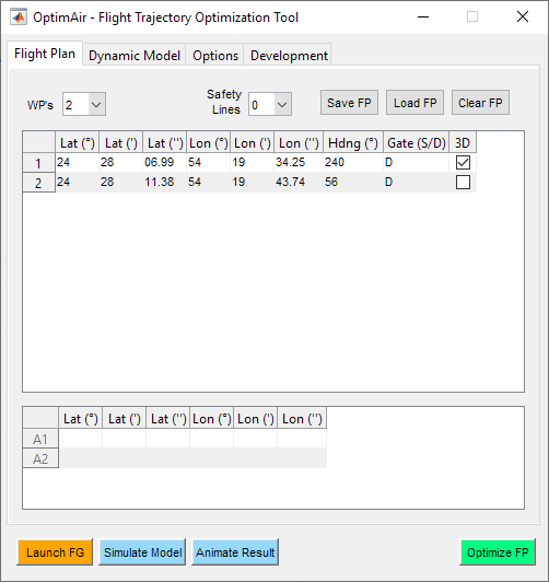
Figure 17 - Flight plan tab
In the Flight Plan tab the user can set the coordinates of the control waypoints, as well as specify if each of those waypoints corresponds to a single or double pylon and if a 3D manouevre (looping) is allowed in that segment. The tool also allows to save flight plans which have already been entered in order to be able to load them directly in the future.
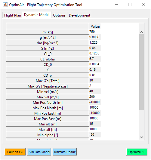
Figure 18 - Dynamic model tab (1)
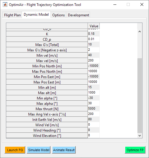
Figure 19 - Dynamic model tab (2)
Dynamic model tab conatins all the configuration parameters related with the aerodynamic derivatives, mass and inertial properties of the aircraft, physical parameters, constraints limits and wind direction and speed.
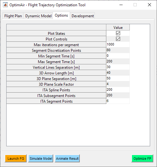
Figure 20 - Options tab
Options tab contains configuration parameters related to the optimization logic, as well as to the plotting capabilities.
Initial trajectory
The quaternion-based model facilitates the convergence to a global minimum by reducing the number of local minima in the solution space. However, in order to increase the probability of achieving this global minimum, it is necessary to provide an initial trajectory which is close to the actual solution. An assistant has been implemented in order to allow the user to set an approximate initial trajectory.
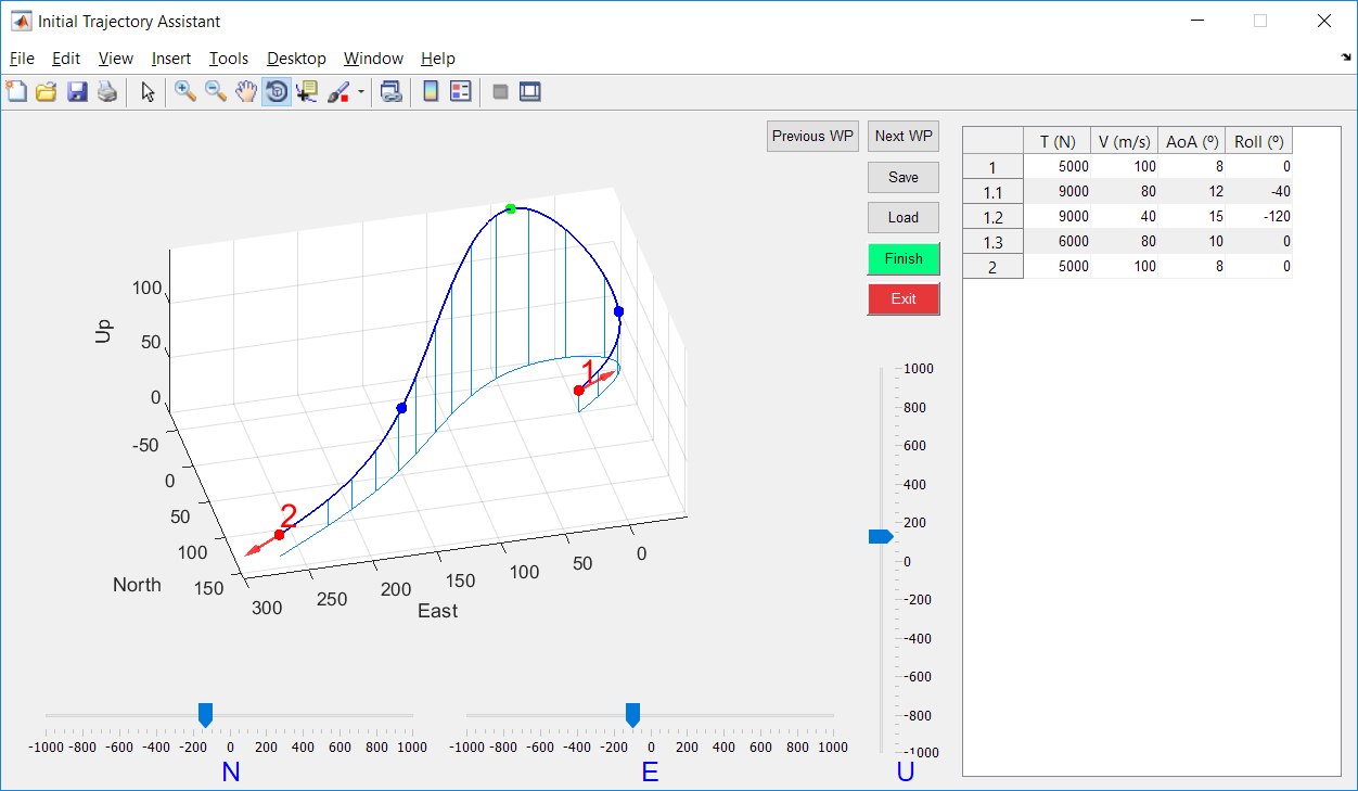
Figure 21 - Initial Trajectory Assistant
The initial trajectory does not only refer to positional trajectory, but also the trajectory of the dynamic states, such as thrust, longitudinal velocity, angle of attack or roll angle. The method of direct collocation for optimal control which falcon.m implements is based on approximating the state history with polynomial splines, so an initial spline should also be provided. State history is entered in the table at the right, specifying the values of the states at each control waypoint. The tool automatically generates splines for this states based on the values entered. One virtual point is appended between each pair of control waypoints (3 virtual points in case the segment has been set as 3D). This virtual points allow to adjust the initial trajectory more precisely.
Optimization
Once everything has been set the tool automatically computes the analytical gradients of the dynamic model using MATLAB Symbolic Toolbox, transforms the optimization problem into a nonlinear programming formulation, compiles this code in C++ using MATLAB Coder toolbox and calls solver Ipopt to execute the optimization process. Here are the results of this simple example (open image in new tab for more detail).
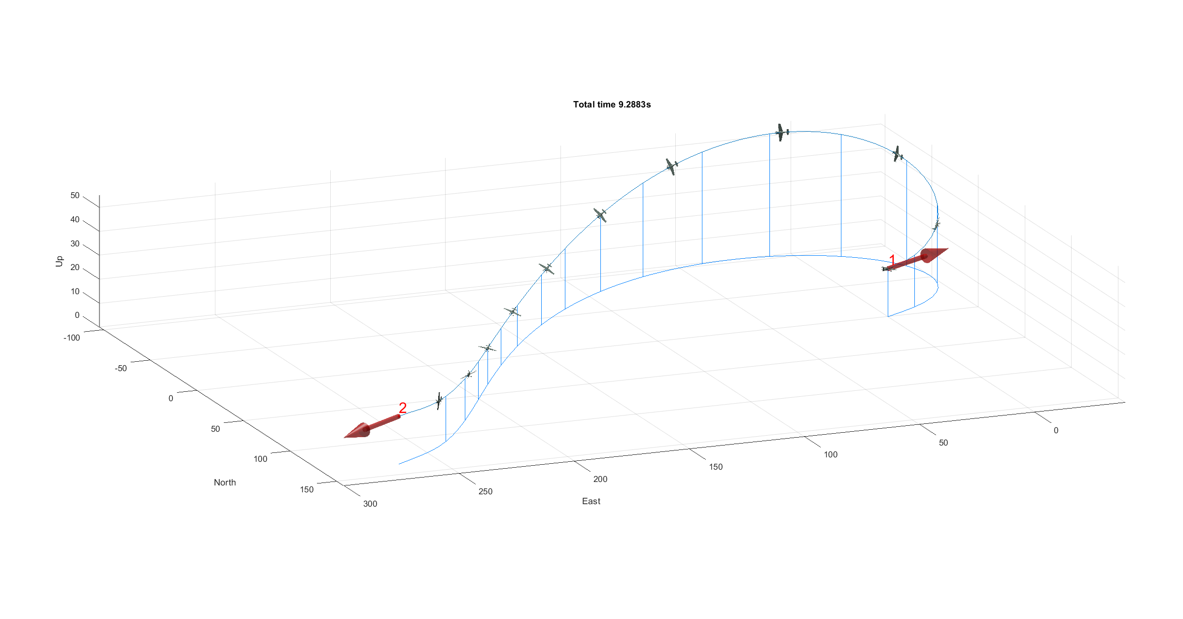
Figure 22 - Optimal trajectory (scale 100%)
The aircraft is represented along the optimal trajectory to help visualizing aircraft attitude along the track. In figure 22 the aircraft is represented at real size, but it can barely be seen. User experience is improved by rendering the aircraft four times bigger than real size (this scale factor can also be adjusted in the Options tab).
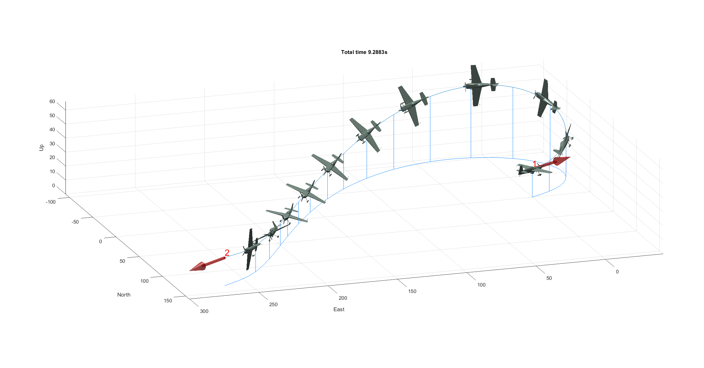
Figure 23 - Optimal trajectory (scale 400%)
Visualization of results
Resulted dynamic states plots are automatically generated and saved in the OutputFiles directory. Roll is shown below as an example.
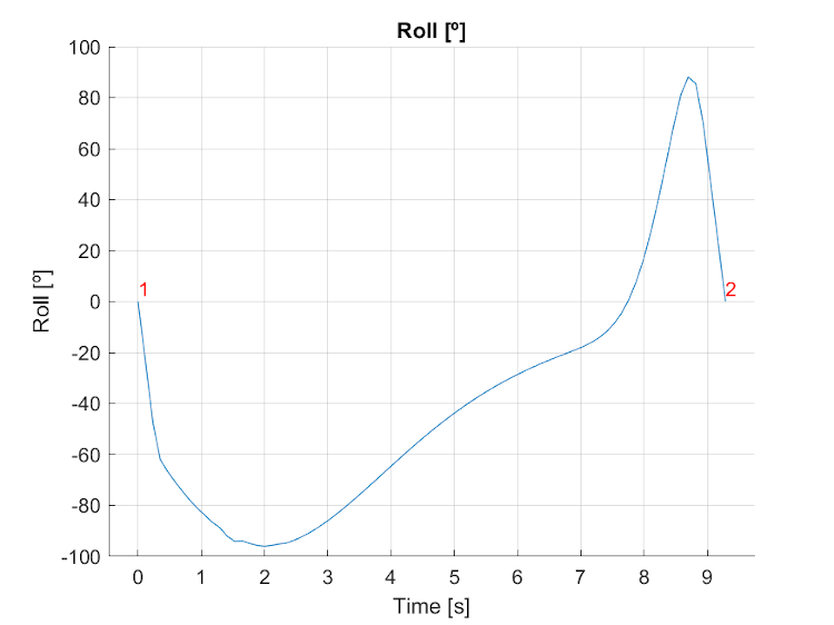
Figure 24 - Roll during optimal trajectory
Additionally, the resulted optimal trajectory can be animated in FlightGear graphical engine by pressing the Animate button at the flight plan tab.
Figure 25 - Optimal trajectory animation in FlightGear
Multiple segments
The simple airtrack segment used in the previous sections corresponds to the 3D segment of Abu Dhabi Red Bull Air Race 2017 track. This optimization was performed on a single segment. Multiple control waypoints can be set in order to perform an optimization of the entire track composed of various segments. An example race track with six control waypoints is shown in the following figures (this track does not correspond with any real track).
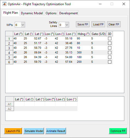
Figure 26 - Multiple segments race track
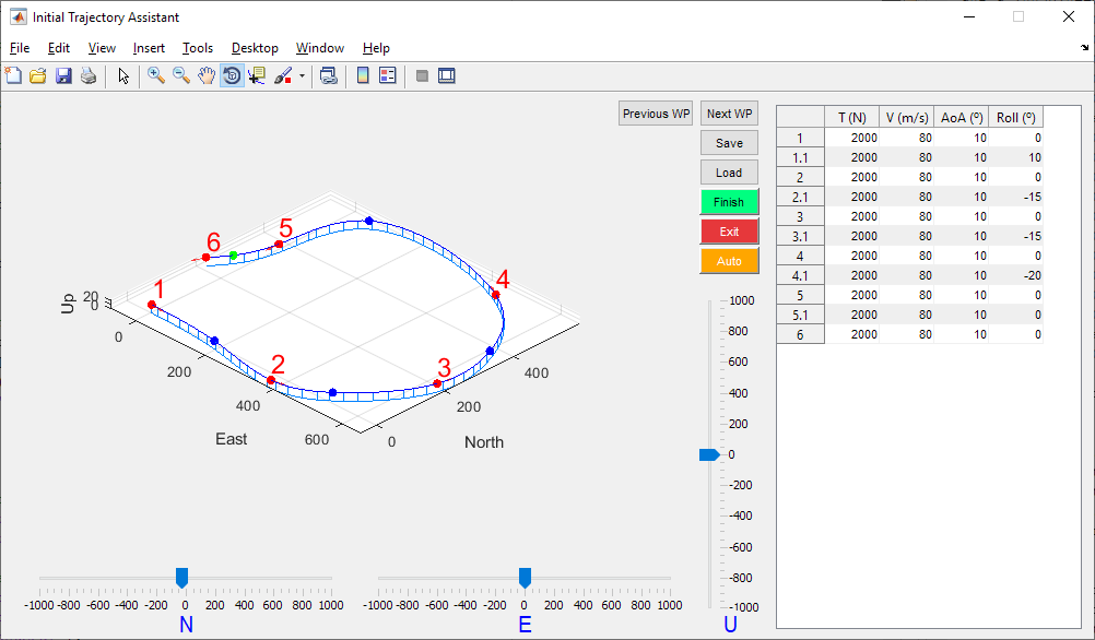
Figure 27 - Initial trajectory assistant
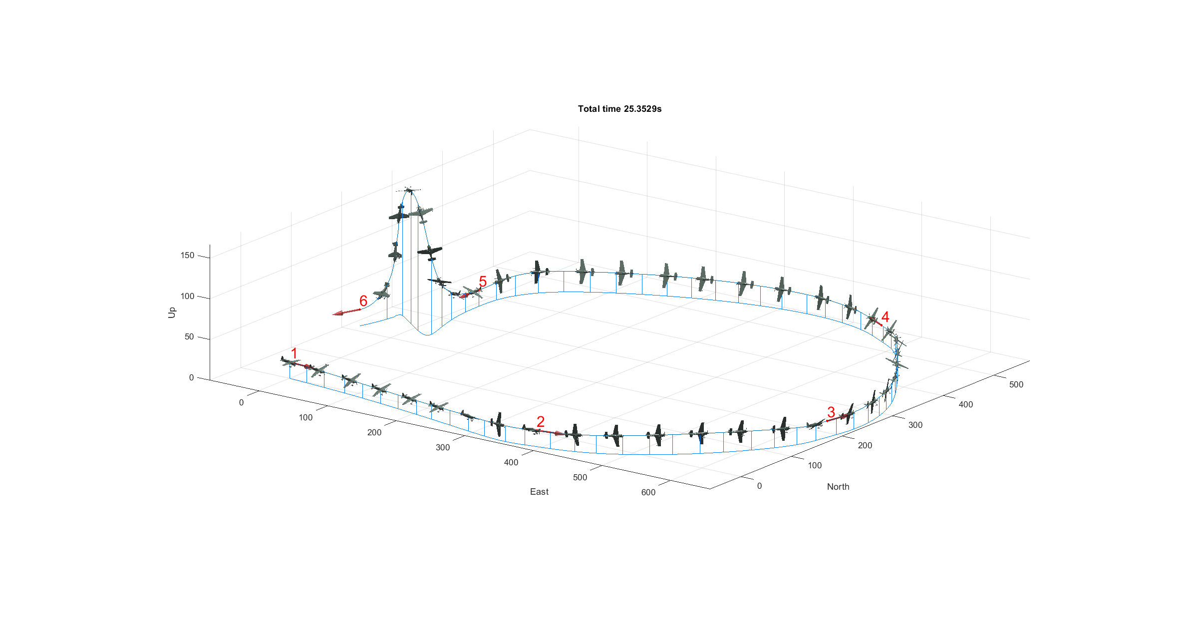
Figure 28 - Optimal trajectory
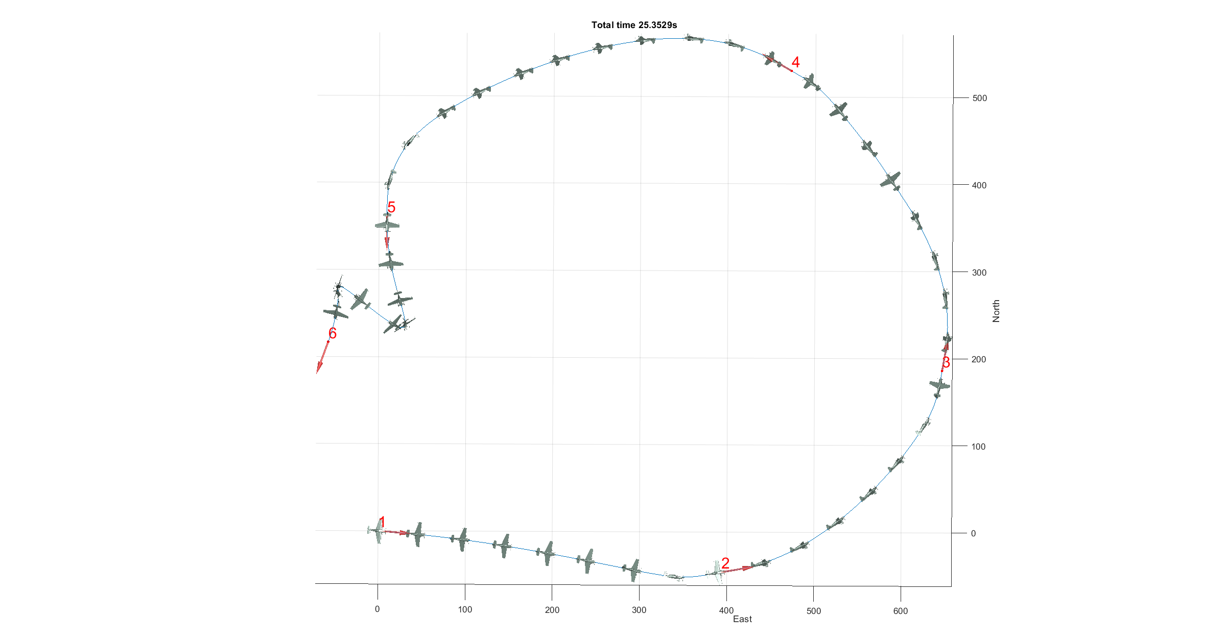
Figure 29 - Optimal trajectory
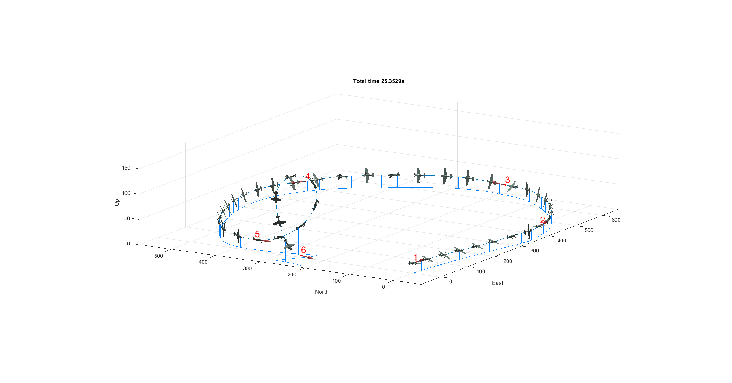
Figure 30 - Optimal trajectory
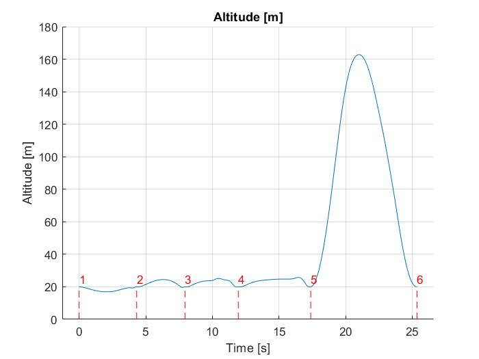
Figure 31 - Altitude profile along optimal trajectory
Safety lines and wind
The tool implements a functionality which allows to introduce up to two safety lines as additional constraints in the optimization problem. A safety line is a segment which delimits the safety area where all the aircraft should remain at all times. Surpassing a safety line during the race implies instant disqualification for the pilot. In the example below, a safety line is introduced in the 3D sector of Abu Dhabi 2017 race track.
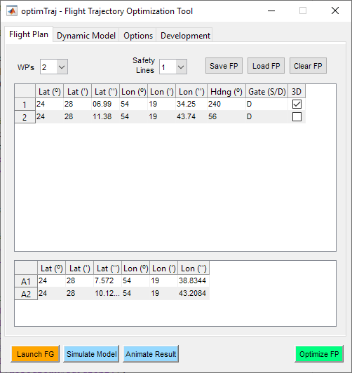
Figure 32 - 3D segment with one safety line
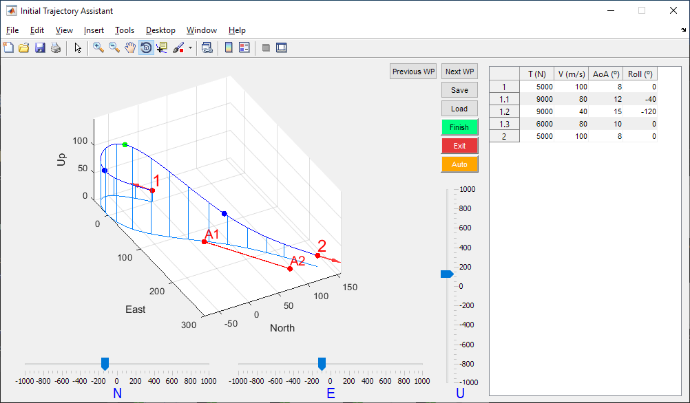
Figure 33 - Initial trajectory assistant
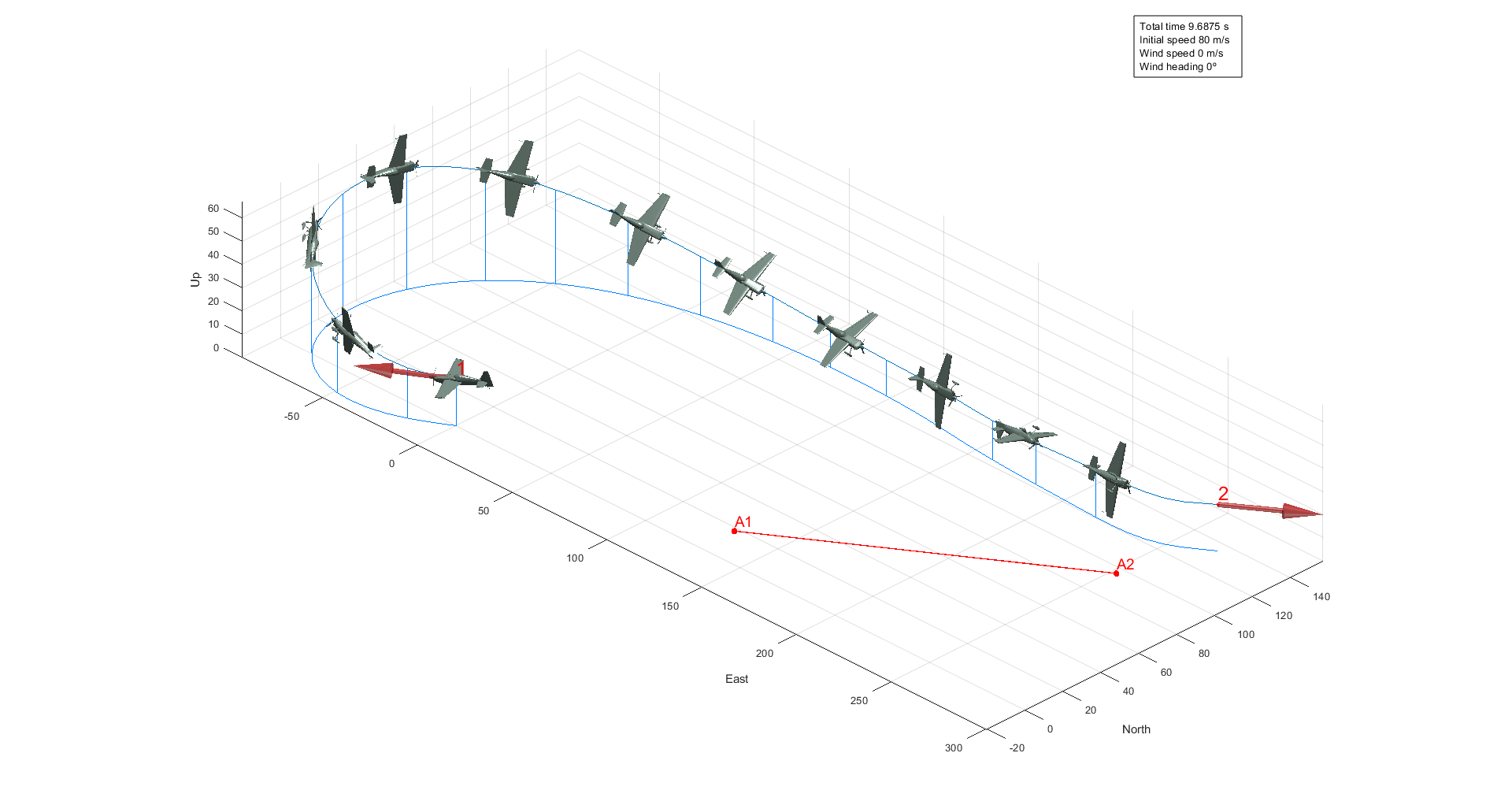
Figure 34 - Optimal trajectory (no wind)
In this situation, a turn towards the right is more optimal, given that the presence of the safety line would force to make a really tight turn towards the left, sacrificing time. However, this is the case if the air is calm. Wind intensity and heading direction can be modified in the options tab. If we introduce some wind the results may vary.
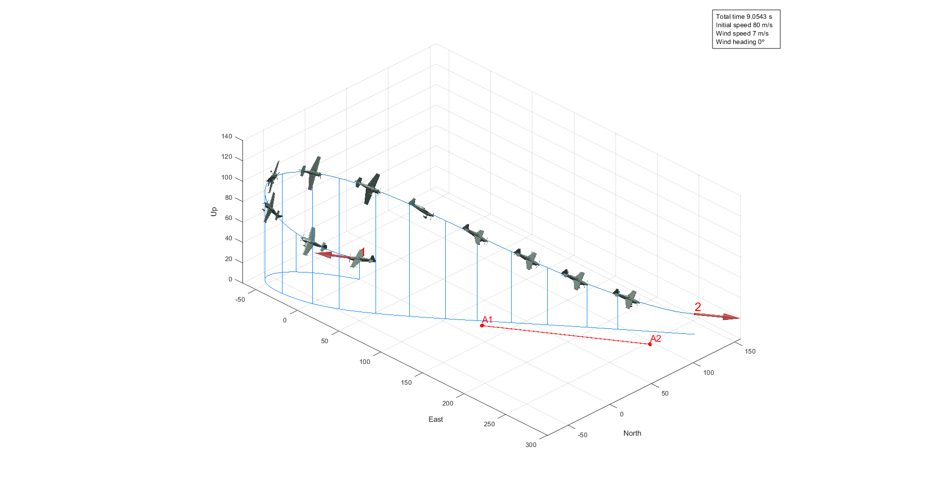
Figure 35 - Optimal trajectory (with wind)
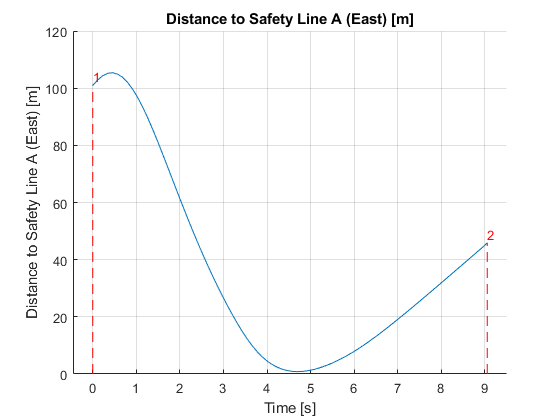
Figure 36 - Distance to safety line along the optimal trajectory
This time the presence of strong winds towards the North make more optimal the turn towards the left, approaching to the safety line area. The optimal trajectory does not surpass the safety line, although it passes really close to it. Although the safety line is defined and represented as a segment, the tool considers the infinite line containing that segment. Up to two simultaneous safety lines can be introduced in the tool (see figure below).
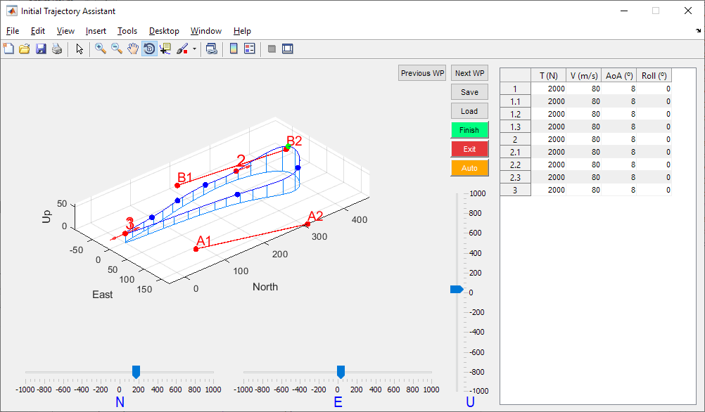
Figure 37 - Initial trajectory for a track with two safety lines
Automatic functionality
The weather forecast for the race day is usually not very precise. This makes an optimization process with different wind speeds, directions and initial velocities really useful. In order to facilitate this iterative process to the user, the tool implements the Auto functionality. When activating this functionality the tool makes multiple optimizations changing the wind velocity and direction inside the specified range. The tool automatically generates images of all the resulting trajectories and states and stores them in a directory structure.
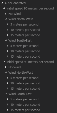
Figure 38 - Automatically generated optimization results directory structure
Each subdirectory contains saved figures of the 3D trajectories, as well as 2D figures of the acceleration, angular velocity, attitude, thrust and position components, and a trajectory timeseries file which can be used to reproduce the trajectory animation in FlightGear. Each of these plots is labelled with its corresponding resulting optimal time, initial speed and wind heading and speed.
Source Code
This application is open-source and licensed under the MIT license. https://github.com/fidelechevarria/OptimAir
References
[1] http://mathworld.wolfram.com/CubicSpline.html
[2] Brian L. Stevens, Frank L. Lewis, and Eric N. Johnson. Aircraft Control and Simulation (3rd ed.). Wiley, 2015.
[3] https://en.wikipedia.org/wiki/Quartic_function
[4] https://www.mathworks.com/discovery/genetic-algorithm.html
[5] https://en.wikipedia.org/wiki/Q-learning#Deep_Q-learning
[6] John T. Betts. Practical Methods for Optimal Control and Estimation Using Nonlinear Programming (2nd ed.). SIAM, 2010.
[7] https://www.fsd.lrg.tum.de/software/falcon-m
[8] A. M. Kuethe and C. Y. Chow. Foundations of Aerodynamics. Wiley, 1984.
[9] https://github.com/coin-or/Ipopt
[10] Hans-Joachim Wuensche. Singularity-free methods for aircraft flight path optimization using euler angles and quaternions. The University of Texas at Austin, Thesis, 1982.
[11] K.H. Well and U. A. Wever. Aircraft Trajectory Optimization using Quaternions - Comparison of a Nonlinear Programming and a Multiple Shooting Approach. Proceedings IFAC 9th Triennial World Congress, Budapest, Hungary, 1984, pp. 1595-1602.
[12] W. G. Breckenridge. Quaternions proposed standard conventions. NASA Jet Propulsion Laboratory, Technical Report, 1979.